

How does AI learn? Training an AI model isn’t magic. It’s a mechanical process: you show the model examples, measure how wrong it is, and adjust its internal knobs to be less wrong. Repeat millions of times, and you get a model that works.
Here’s the machinery underneath.
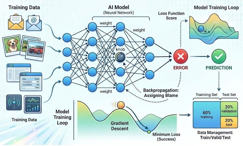
The Training Pipeline: Data to Model
Before training even starts, you need a plan for your data.
You collect raw data (emails, images, transactions, sensor readings—whatever your problem requires). You clean it (remove garbage, fix errors, handle missing values). You normalize it (scale numbers to a consistent range so the model doesn’t get confused by different units). Then you split it into three parts: a training set, a validation set, and a test set.
The training set is what the model learns from. You show it thousands of examples, and the model adjusts itself based on what it sees.
The validation set is a referee. While training happens, you periodically check the model against data it’s never seen before. If the model is overfitting—memorizing training examples instead of learning general patterns—the validation set will catch it. The model never learns from validation data; it’s only for observation.
The test set is a final exam. You keep it locked away until training is completely done. Only then do you measure the model’s real-world accuracy on data it’s truly never encountered.
This separation is critical. If you test on the same data the model was trained on, you’ll get an inflated score that doesn’t reflect how the model will perform on new problems.
Loss Functions: The Scoreboard
How does the model know it’s wrong?
A loss function measures how bad the model’s predictions are. The lower the loss, the better the model. Different problems use different loss functions.
For a spam filter, the loss might be: “How many emails did you misclassify?” If the model predicts “spam” for an email that’s actually legitimate, the loss goes up.
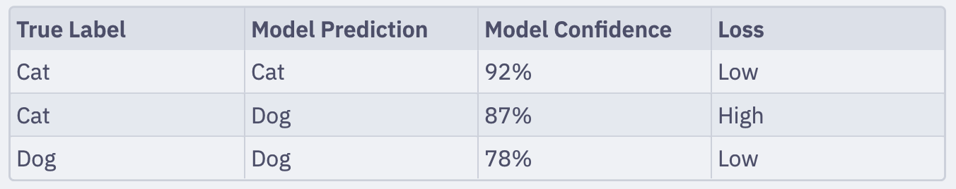
For an image classifier that identifies dog breeds, the loss might measure the probability distance between the predicted label and the true label. If the model is 90% confident it’s a poodle but it’s actually a dachshund, the loss is high. If it’s 95% confident it’s a dachshund, the loss is lower.
Here’s a concrete example:
Gradient Descent: Rolling Downhill
Now, how does the model actually adjust itself?
Imagine you’re blindfolded at the top of a hill, trying to reach the lowest point. You can’t see the whole landscape. You feel the slope under your feet, and you take a small step downhill. Then you check the slope again and take another step. Repeat long enough, and you’ll reach a valley.
Gradient descent is this process. The model calculates the slope of the loss function with respect to each of its parameters (called the “gradient”). Then it takes a small step in the direction that reduces loss. It does this thousands or millions of times.
The word “gradient” sounds fancy but it just means: “In which direction does the loss go down, and how steep is it?”
Backpropagation: Assigning Blame
Gradient descent needs to know which parameters to adjust. This is where backpropagation comes in.
Backpropagation is the mechanism that calculates how much each internal parameter contributed to the error. It works backward from the output, asking: “How did this layer’s weights affect the mistake? And the layer before that?”
Think of it as an error audit trail. If the model predicted 95 instead of 50, backpropagation traces the error backward through every calculation and says, “This weight contributed 3 to the error. That weight contributed 7. This one contributed -2.” Gradient descent then adjusts these weights based on their contributions.
You don’t need to understand the mathematics to use it. The key insight: backpropagation lets the model figure out what to fix.
Epochs and Batch Size: The Training Rhythm
Training happens in cycles.
An epoch is one full pass through the entire training dataset. If you have 10,000 training examples, one epoch means the model has seen all 10,000 exactly once.
But you don’t show the model all 10,000 at once. You show them in groups called batches. A batch size of 32 means you process 32 examples, calculate their total loss, backpropagate, adjust the weights, then move to the next 32. This happens because processing one example at a time is slow, and processing all of them at once requires too much memory.
A typical training run might look like: 100 epochs, batch size 32. The model sees all training data 100 times, processing it in batches of 32 each time. Loss decreases with each epoch until it plateaus. That’s when you stop.
Data Quality Beats Algorithm Quality
Here’s something instructors wish beginners knew: better data beats better algorithms.
You can have the fanciest, most sophisticated model ever designed. But if your training data is garbage—full of errors, biased, or unrepresentative of the real world—the model will be garbage. Conversely, mediocre algorithms trained on clean, representative data often outperform fancy algorithms trained on messy data.
This is why data preparation takes longer than algorithm selection in real projects. And why data engineers are in high demand.
The Trust Boundary: Training as a Security Gate
The training process is a boundary where trust matters.
If someone poisons your training data—inserting malicious examples or corrupting labels—the model learns the poisoned patterns. It becomes a poisoned model. The model doesn’t know it learned the wrong thing. It’s confident. It just works based on what it saw.
This is especially dangerous with self-supervised learning and large language models. An LLM trained on poisoned text learns “facts” that are false, and those falsehoods get baked into billions of parameters. The model has “memorized” the corruption.
This is why training data provenance (knowing where it came from and who had access to it) matters in security-critical applications.
Bringing It Together
Training is straightforward in outline: prepare data → measure loss → calculate gradients → adjust weights → repeat. But this simple loop, repeated millions of times on billions of examples, produces systems that can recognize patterns humans barely see.
The key to good models isn’t fancy mathematics. It’s clean data, a sensible loss function, and patience.